Animating simple cellular automata with Python
Learn how to combine Python’s scientific stack with MoviePy to animate spaceships, oscillators, guns and expanding mazes.
Recently, I had a talk on Prim’s algorithm at a meeting of our local algorithmic club. While preparing for the talk, I created several animations of the maze generating process using matplotlib. I can’t say it was a fun time. Animating several thousands of frames took ages, not to mention that the API is rather low-level.
Agreed, matplotlib is well suited for producing short animations of plots, but for combining a large number of images into a movie or animated GIF I needed to find another tool. I looked around and found an excellent MoviePy library.
At the next meeting of our club, we will be delving deeper into generating mazes, this time using cellular automata. This makes it a perfect opportunity to describe here how one can implement such automata in Python and visualize their evolution with beautiful video clips produced by MoviePy.
Here’s what you’ll find in today’s post.
- Introduction to cellular automata.
- Counting neighbours as a 2D convolution
- Implementing evolution of cellular automata using numpy stack
- Drawing state of an automaton using matplotlib
- Creating animation of evolving automata using MoviePy
- Gallery of nice examples produced by our scripts
Prerequisites
To run the examples from this post you’ll need several packages. I used Python 3.7 with:
scipy1.3.1numpy1.17.3matplotlib3.0.2moviepy1.0.1
Introduction to cellular automata
Consider a square grid, where each cell can be in one of some predefined states. For this post we will restrict ourselves to automata with only two possible states, that is a cell can be either alive or dead. To each cell, one can assign its neighbourhood, i.e. set of cells that are directly in contact (via border or a corner) with it. The figure below shows a 4x5 grid with a red cell along with its neighbours.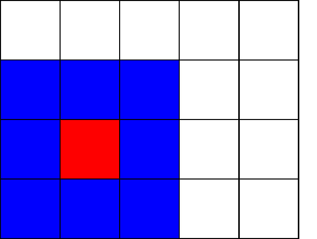
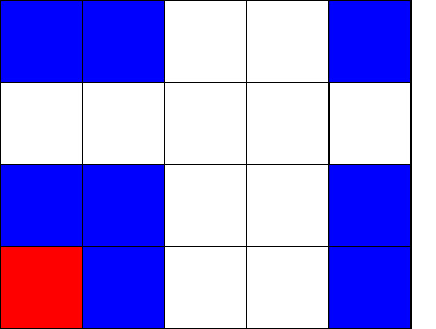
Note the special case of the cells lying at the edge or in the corner of the grid. We have basically two choices:
- considering only the “real” neighbours. In this approach, the neighbourhood of such cells is smaller than that of ones lying in the interior.
- virtually connecting the opposite edges. This wraps our grid, making it a torus.
Below we can see how the neighbourhood of the corner cell looks like depending whether we wrap the grid or not.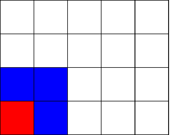
We start with some initial state of each cell in the grid. We can transform the grid by applying a set of rules determining the next state of each cell as a function of its neighbours’ states.
For instance, the set of rules below defines a cellular automaton known as Conway’s Game of Life:
- If a dead cell has at least three neighbours, it becomes alive.
- If an alive cell has two or three neighbours it stays alive.
- All other alive cells become dead. That is, cells with less than two or more than four alive neighbours die.
One can see how the above rules describe a very simplified evolution of some primitive population. Each member of the population needs just the right number of neighbours to survive, otherwise, it dies as a result of under- or overpopulation. New members of the population may also be born if the conditions are favourable.
If we restrict ourselves only to rules based on the number of neighbours, the behaviour of automaton can be completely specified by its initial state and two lists:
- list of numbers of neighbours defining when the dead cell becomes alive (in Game of Life this is [3]),
- list of numbers of neighbours defining when the living cell survives (in Game of Life this is [2, 3]).
Cells that are not born and do not survive can be considered dead since they either were dead before and haven’t become alive, or they died because they didn’t match survival criterion. One can write the rules concisely using a so-called rule string. There exist several formats of rule strings, but probably the most widely used takes the form Bx/Sy, where x denotes all numbers from the first list and y denotes all numbers from the second one. For instance, in this notation the rule string for Game of Life is B3/S23.
It would be now straightforward to implement a simple automaton using Python. However, before we do that, let’s discuss an alternative view on the neighbour-counting process that will allow us to vectorize some computations.
Counting neighbours as a 2D convolution
Let’s represent our grid as a matrix with 0s and 1s marking dead and alive cells respectively. Our goal is to produce a matrix with the same size as an input grid, but with all entries equal to the number of alive neighbours of the corresponding cell. For instance, assuming that we don’t wrap edges, this is an example of transformation we wish to perform:
And here is how the same transformation looks like if we glue the opposite edges:
Let’s forget about the edge cells for a moment and focus only on the ones in the interior. It turns out that for those cells the process boils down to the following steps:
Define matrix $K$: \[K = \begin{bmatrix} 1 & 1 & 1 \\ 1 & 0 & 1 \\ 1 & 1 & 1 \end{bmatrix}\]
- Create an empty matrix $M$ of the same size as an input grid.
- For each cell in the interior of the input grid:
- Position matrix $K$ on top of the input grid such that the current cell lies below $0$.
- Multiply elements of $K$ with corresponding elements of the grid.
- Sum the results of this multiplication and place it in the corresponding place in $M$.
See the equation below for an example of the above process.
As you may already see, what we perform here is a 2D convolution of our grid with $K$ as a kernel. Note that normally when performing convolution we reverse the order of rows and columns in a kernel, but $K$ is invariant under such reversal.
This is great because 2D convolution is already implemented in SciPy stack. Indeed, running the following code produces the result as in the example above.
import numpy as np
from scipy.signal import convolve2d

kernel = np.array([
    [1, 1, 1],
    [1, 0, 1],
    [1, 1, 1]
])
grid = np.array([
    [0, 1, 0, 1],
    [1, 1, 1, 0],
    [0, 0, 1, 0],
    [1, 0, 1, 0]
])

result = convolve2d(grid, kernel, mode="same", boundary="fill")
print(result)
[[3 3 4 1]
 [2 4 4 3]
 [3 6 3 3]
 [0 3 1 2]]
The mode="same" tells convolve2d to return an array of the same shape as the grid, otherwise, the full output larger than the grid is returned. Specifying boundary determines how the boundary cells are handled. There are several options, but the ones we are interested in are the following:
"fill": virtually extend the grid (by default with zeros), so the convolution can be performed as for interior elements."wrap": glue opposite edges of the grid together.
Now that we know all the necessary tools, we can move on to the actual implementation of our automata.
Implementing evolution of cellular automata using numpy
Let us first write down the requirements for our implementation. While it might be tempting to write a class like CellularAutomaton, I think a cleaner solution is to just write a generator the yields consecutive states of the grid. What input data do we need?
- An initial state of the grid.
- The rules (specified by a rule string).
- A boolean indicating whether we should wrap the edges.
Therefore, our generator could have a signature like this:
def evolve(initial_state: np.ndarray, rules: str, wrap: bool = False) -> np.ndarray:
    pass
Before we implement it, however, let’s write a simple helper that parses a rule string and produces two lists of integers - numbers of neighbours needed for birth and survival of a cell.
import re
from typing import List, Tuple


def parse_rules(rule_string: str) -> Tuple[List[int], List[int]]:
    match = re.match(r"B(\d*)/S(\d*)", rule_string)
    return tuple([int(char) for char in group] for group in match.groups())
A function for parsing a rule string. For simplicity, we assume that the input string is correct and don’t perform any error checking.
This is pretty simple:
- We first match the input string to the suitable regular expression. This expression matches exactly those strings that have a letter B, followed by some number of digits, then by a slash, then by a letter S and finally again by some number of digits. Note that any of the groups of digits can be empty because we used
*instead of+. - If the expression matched, we have exactly two groups in the match - they correspond to the first and the second sequence of digits.
- We convert each digit in those two groups into an integer, and in the end, return two lists of numbers.
Now let’s see how to evolve the grid. If we had boolean arrays marking the newly born cells and the surviving cells, then the new state is simply a logical elementwise or between them. Obtaining those arrays is straightforward using NumPy’s isin function, which is a vectorized version of the built-in in operator. The following example shows how it works.
import numpy as np

arr = np.array([[1, 0, 2], [4, 2, 1]])

print(np.isin(arr, [1, 2]))
[[ True False  True]
 [False  True  True]]
NumPy isin function in action. The output array has the same shape as arr, and each of its entry tells whether the corresponding element in arr is equal to 1 or 2.
A boolean array marking newly cells can be constructed as follows:
- Compute an array with neighbour counts.
- Using
isin, construct a boolean array marking cells that have sufficient neighbours to be born. - Use logical
andto combine this boolean array with the negation of the current grid.
The last step is necessary because only the cells that were previously dead can be born. Marking surviving cells is similar, the only significant difference is that we combine it with the grid instead of its negation (because only already living cells can survive).
Here’s how the code for evolving our automaton might look like.
from functools import reduce
import numpy as np
from scipy.signal import convolve2d


def evolve(initial_state: np.ndarray, rules: str, wrap: bool = False) -> np.ndarray:
    birth_list, survival_list = parse_rules(rules)
    kernel = np.array([[1, 1, 1], [1, 0, 1], [1, 1, 1]])
    grid = np.array(initial_state)
    boundary = "wrap" if wrap else "fill"
    while True:
        yield grid
        neighbours = convolve2d(grid, kernel, mode="same", boundary=boundary)
        birth_mask = np.isin(neighbours, birth_list)
        survival_mask = np.isin(neighbours, survival_list)
        grid = (birth_mask & ~grid) | (survival_mask & grid)
We can easily verify that the above code produces correct results, but it would require manual inspection of the produced arrays. This is quite boring, so let’s focus on visualizing our automata.
Drawing state of an automaton using matplotlib
Drawing state of our automaton is simple. Basically, we draw our image using imshow and add grid positioned at half-integer marks. We also remove any other elements like spines and tick labels.
from matplotlib import pylab as plt
from matplotlib.cm import binary

def plot_state(state, axes, line_width=2):
    axes.imshow(state, interpolation="none", cmap=binary, zorder=0)
    axes.set_xticks(np.arange(-0.5, state.shape[1]+0.5, 1), minor=True)
    axes.set_yticks(np.arange(-0.5, state.shape[0]+0.5, 1), minor=True)
    axes.yaxis.grid(True, which='minor', linewidth=line_width)
    axes.xaxis.grid(True, which='minor', linewidth=line_width)

    for spine in ["left", "right", "top", "bottom"]:
        axes.spines[spine].set_visible(False)

    for axis in (axes.xaxis, axes.yaxis):
        axis.set_ticklabels([])
        axis.set_ticks_position('none')
A function plotting state of an automaton to matplotlib Axes object. Notice the use of z-order in imshow call.
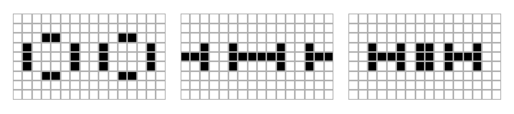
In the below script we utilize plot_state function to plot several states of some automaton.
from itertools import islice

initial_state = np.array(
    [
        [0, 0, 0, 0, 0, 0, 0, 0, 0, 0, 0, 0, 0, 0, 0, 0],
        [0, 0, 0, 0, 0, 0, 0, 0, 0, 0, 0, 0, 0, 0, 0, 0],
        [0, 0, 0, 0, 0, 0, 0, 0, 0, 0, 0, 0, 0, 0, 0, 0],
        [0, 0, 0, 0, 0, 1, 0, 0, 0, 0, 1, 0, 0, 0, 0, 0],
        [0, 0, 0, 1, 1, 0, 1, 1, 1, 1, 0, 1, 1, 0, 0, 0],
        [0, 0, 0, 0, 0, 1, 0, 0, 0, 0, 1, 0, 0, 0, 0, 0],
        [0, 0, 0, 0, 0, 0, 0, 0, 0, 0, 0, 0, 0, 0, 0, 0],
        [0, 0, 0, 0, 0, 0, 0, 0, 0, 0, 0, 0, 0, 0, 0, 0],
        [0, 0, 0, 0, 0, 0, 0, 0, 0, 0, 0, 0, 0, 0, 0, 0],
    ]
)

states = list(islice(evolve(initial_state, "B3/S23"), 8, 11, None))

fig, axes = plt.subplots(1, 3, figsize=(16, 3))

for state, axis in zip(states, axes):
    plot_state(state, axis)

plt.show()
Example usage of plot_state function. Notice that using islice we take only three states of the automaton, starting at the eighth one. Size of the figure has been chosen purely arbitrarily (it looked quite appealing in my jupyter notebook).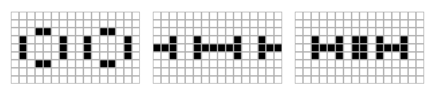
This looks pretty nice, but it would be much nicer if we created an animated sequence of images or a movie clip of the automaton progressing through its states, which is what we’ll do next.
Creating animation of evolving automata using MoviePy
To produce an animation using MoviePy we first need to create a list of frames that will be combined into a single clip. We could construct required frames ourselves using figure’s canvas tostring_rgb() method but luckily MoviePy has us covered and provides mplfig_to_npimage specifically for that purpose.
Once we have a list of frames, we use it to initialize an instance of ImageSequenceClip. In turn, this instance can be used to produce an animated gif or video file, or even displayed in Jupyter Notebook. The process is shown in the snippet below.
from itertools import islice
from moviepy.editor import ImageSequenceClip
from moviepy.video.io.bindings import mplfig_to_npimage

def animate_automaton(
    states: np.ndarray, line_width=2, fps=2, **fig_kwargs
) -> ImageSequenceClip:
    fig, axes = plt.subplots(1, 1, **fig_kwargs)

    frames = []

    for state in states:
        plot_state(state, axes, line_width=line_width)
        frames.append(mplfig_to_npimage(fig))

    return ImageSequenceClip(frames, fps=fps)


initial_state = np.array([
    [0, 0, 0, 0, 0, 0, 0, 0, 0, 0, 0, 0, 0, 0, 0, 0],
    [0, 0, 0, 0, 0, 0, 0, 0, 0, 0, 0, 0, 0, 0, 0, 0],
    [0, 0, 0, 0, 0, 0, 0, 0, 0, 0, 0, 0, 0, 0, 0, 0],
    [0, 0, 0, 0, 0, 1, 0, 0, 0, 0, 1, 0, 0, 0, 0, 0],
    [0, 0, 0, 1, 1, 0, 1, 1, 1, 1, 0, 1, 1, 0, 0, 0],
    [0, 0, 0, 0, 0, 1, 0, 0, 0, 0, 1, 0, 0, 0, 0, 0],
    [0, 0, 0, 0, 0, 0, 0, 0, 0, 0, 0, 0, 0, 0, 0, 0],
    [0, 0, 0, 0, 0, 0, 0, 0, 0, 0, 0, 0, 0, 0, 0, 0],
    [0, 0, 0, 0, 0, 0, 0, 0, 0, 0, 0, 0, 0, 0, 0, 0],
])

states = list(islice(evolve(initial_state, "B3/S23"), 15))

clip = animate_automaton(states, figsize=(16, 9), dpi=30, fps=2, line_width=4)

clip.write_gif("automaton.gif")
Animating cellular automaton using moviepy. Here we use islice to select only first fifteen first states of the evolution. The write_gif method is used to save our animation as a gif, alternatively write_videofile could be used to save animation as a video file. {.:figcaption}
Gallery of examples
Depite their simplicity, behaviour of cellular automata can be surprisingly rich and complex. So, to conclude, lets see some nice example animations.