Computing highly oscillating integrals using Python
Getting most of Python’s numerical libraries when integrating wildly oscillating integrals
Recently during my research I stumbled upon the following indefinite integral that needed to be computed for various values of $\omega \in (0, \infty)$. Well, maybe not precisely this integral but a really similar one. Anyway here it goes: \[I(\omega) = \int_0^\infty x\exp(-x)cos(\omega x) dx.\]
Naively, I just threw it into scipy.integrate.quad routine. For small values of $\omega$ it works fine, but as $\omega$ gets larger we run into troubles - run the below code and see for yourself.
from numpy import exp, tanh, cos, inf
from scipy.integrate import quad

OMEGA = 30

def func(x):
    if x == 0:
        return 1
    else:
        return x * exp(-x) / tanh(x) * cos(OMEGA * x)

print(quad(func, 0, inf))
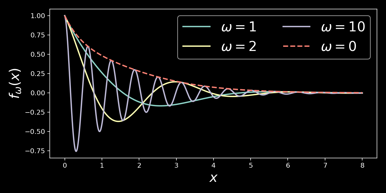
You may see the integrand for various values of $\omega$ in below plot.
Clearly this integral is convergent so why does numerical integrator fail? The reason lies in the oscillating nature of the integrand. It is often the case that highly oscillating integrals require special treatment and this is what we are going to discuss today.
Taming oscillating integrands using Python
Solution using scipy
Unsurprisingly quad can deal with our integral - we just need to feed it right parameters. The key to the solution is treating our integral as a weighted one. It turns out that if your integrand is of the form $f(x)g(\omega x)$, where $g$ is either $sin$ or $cos$, scipy (or rather: quadpack that is used under the hood) can compute it using a quadrature specifically taiored to deal with such problems.
So, computing the above integral can be done in scipy as follows
from numpy import exp, tanh, inf
from scipy.integrate import quad

OMEGA = 30

def func(x):
    return 1 if x == 0 else x * exp(-x) / tanh(x)

result, err = quad(func, 0, inf, weight='cos', wvar=OMEGA)

print('Result: {0}, error: {1}'.format(result, err))
Pretty simple!
Solution using mpmath
The mpmath package has a function quadosc for the sole purpose of computing integrals of oscillating functions (docs here). The usage is simple, you need to pass quadosc a function to integrate, integration limits and either the angular frequency (the $\omega$ in our function) or period of oscillatory term.
from mpmath import exp, tanh, cos, quadosc, inf

OMEGA = 30

def func(x, omega):
    if x == 0:
        return 1
    else:
        return x * exp(-x) / tanh(x) * cos(omega * x)

integrand = lambda x: func(x, OMEGA)
result = quadosc(integrand, [0, inf], omega=OMEGA)
print('Result: {}'.format(result))
Which one to choose?
If we rrun both of the above examples we will see that they give similar results. So which approach to choose? There are two factors to consider: speed and accuracy.
To analyse speed of scipy.quad and mpmath.quadosc I computed our integral for multiple values of $\omega$ between 1 and 100, 100 times for each value using both methods. The below plot shows mean time to solution, y-axis in log scale.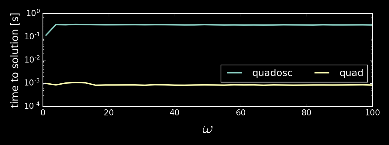
As we may see using quad is almost three orders of magnitude faster than quadosc.
Ok, so scipy is faster here. But what about accuracy? It is hard to measure it for our integrand, as we don’t know the exact solution. Let’s compute another integral, one which we can solve analytically, namely: \[F(\omega) = \int_0^\infty x\exp(-x)cos(\omega x) dx.\]
We can easily compute the above integral explicitly (nice exercise if you haven’t computed any integrals for some time!). The exact solution is $F(\omega) = \omega / (\omega^2 + 1)$. I computed the $F(\omega)$ numerically for various values of $\omega$ between 1 and 100. The below plot shows errors of numerical results with respect to the exact solution.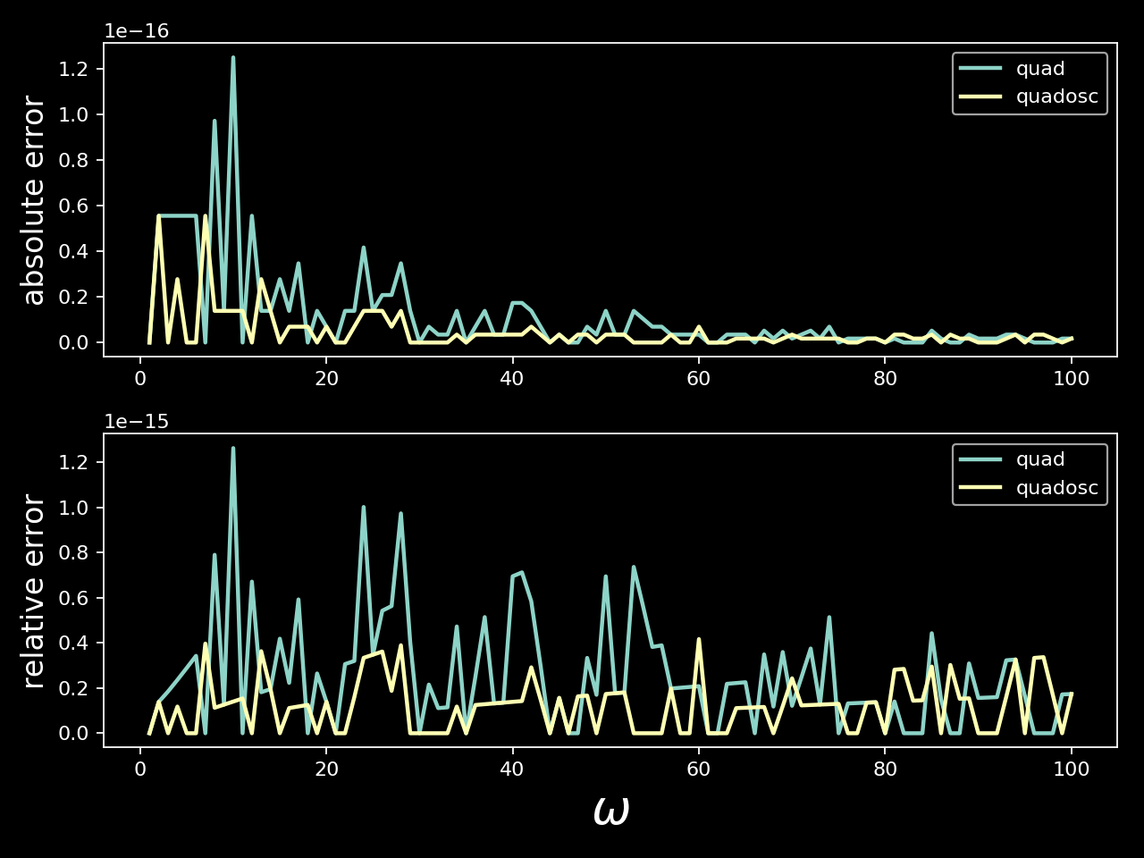
Although quadosc gives slightly smaller error, the differences are neglible, relative errors as well as absolute ones are small for boths methods.
It seems that quad is a clear winner, offering comparable accuracy of solution in much better time.
What about mpmath.quad?
Documentation states that for exponentially or faster decaying integrals mpmath.quad should work equally fine as mpmath.quadosc and should be much faster. I tried it for $F(\omega)$ and it performed much worse than other solutions presented above. Below plot shows error of $F(\omega)$ values computed using mpmath.quad with respect to exact solution.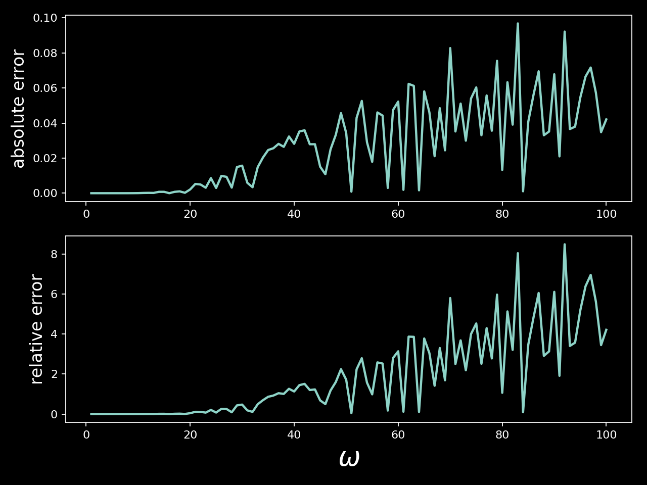
As can be seen, mpmath.quad doesn’t work well when oscillation frequency increases. For large values of $\omega$ the relative error reaches as high as 800%.
Summary
We presented two methods for integrating higly oscillating functions using Python scientific libraries. Both mpmath.quadosc and scipy.integrate.quad gave accurate results for the tested function, however quad outperformed quadosc in terms of timing.
In interpreting results of our small benchmark we should note that mpmath.quadosc offers more flexibility when defining oscillatory terms. In particular, it offers the following possibilities that were not exploited in the benchmark:
- computing integral with oscillating term different than $\cos$ and $\sin$
- computing integrals wich uneven oscillations (for instance with oscillatoring term $\sin(x^2)$)
Keeping that in mind, mpmath.quadosc should still be regarded as an useful tool, but for the problem discussed in this post it falls behind scipy.integrate.quad.
The final thing to consider is that I run all of the benchmarks without tweaking any of the additional parameters of the used integrators. It is possible that better results, either in terms of accuracy or timing, can be achieved if such fine tuning is performed. The reason I didn’t dwelve into this too much is primarily because I didn’t have time to perform extensive studies. Secondly, I think that a tool is most valuable if you can use it without too much tweaking. Therefore it is good to see what numerical integrators can do with their default settings.